Epilepsy Detection Using EEG Data
IPython notebook: download
In this example we’ll use the cesium library to compare
various techniques for epilepsy detection using a classic EEG time series dataset from
Andrzejak et al..
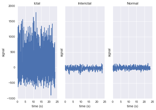
The raw data are separated into five classes: Z, O, N, F, and S; we will consider a
three-class classification problem of distinguishing normal (Z, O), interictal (N, F), and
ictal (S) signals.
The overall workflow consists of three steps: first, we “featurize” the time series by selecting some set of mathematical functions to apply to each; next, we build some classification models which use these features to distinguish between classes; finally, we validate our models by generating predictions for some unseen holdout set and comparing them to the true class labels.
First, we’ll load the data and inspect a representative time series from each class:
%matplotlib inline
import numpy as np
import matplotlib.pyplot as plt
import seaborn; seaborn.set()

from cesium import datasets

eeg = datasets.fetch_andrzejak()

# Group together classes (Z, O), (N, F), (S) as normal, interictal, ictal
eeg["classes"] = eeg["classes"].astype('U16') #  allocate memory for longer class names
eeg["classes"][np.logical_or(eeg["classes"]=="Z", eeg["classes"]=="O")] = "Normal"
eeg["classes"][np.logical_or(eeg["classes"]=="N", eeg["classes"]=="F")] = "Interictal"
eeg["classes"][eeg["classes"]=="S"] = "Ictal"

fig, ax = plt.subplots(1, len(np.unique(eeg["classes"])), sharey=True)
for label, subplot in zip(np.unique(eeg["classes"]), ax):
    i = np.where(eeg["classes"] == label)[0][0]
    subplot.plot(eeg["times"][i], eeg["measurements"][i])
    subplot.set(xlabel="time (s)", ylabel="signal", title=label)
Featurization
Once the data is loaded, we can generate features for each time series using the
cesium.featurize
module. The featurize module includes many built-in choices of features which can be applied
for any type of time series data; here we’ve chosen a few generic features that do not have
any special biological significance.
If Celery is running, the time series will automatically be split among the available workers
and featurized in parallel; setting use_celery=False will cause the time series to be
featurized serially.
from cesium import featurize
features_to_use = ['amplitude',
                   'percent_beyond_1_std',
                   'maximum',
                   'max_slope',
                   'median',
                   'median_absolute_deviation',
                   'percent_close_to_median',
                   'minimum',
                   'skew',
                   'std',
                   'weighted_average']
fset_cesium = featurize.featurize_time_series(times=eeg["times"],
                                              values=eeg["measurements"],
                                              errors=None,
                                              features_to_use=features_to_use,
                                              targets=eeg["classes"], use_celery=True)
print(fset_cesium)
<xarray.Dataset>
Dimensions:                    (channel: 1, name: 500)
Coordinates:
  * channel                    (channel) int64 0
  * name                       (name) int64 0 1 2 3 4 5 6 7 8 9 10 11 12 13 ...
    target                     (name) object 'Normal' 'Normal' 'Normal' ...
Data variables:
    minimum                    (name, channel) float64 -146.0 -254.0 -146.0 ...
    amplitude                  (name, channel) float64 143.5 211.5 165.0 ...
    median_absolute_deviation  (name, channel) float64 28.0 32.0 31.0 31.0 ...
    percent_beyond_1_std       (name, channel) float64 0.1626 0.1455 0.1523 ...
    maximum                    (name, channel) float64 141.0 169.0 184.0 ...
    median                     (name, channel) float64 -4.0 -51.0 13.0 -4.0 ...
    percent_close_to_median    (name, channel) float64 0.505 0.6405 0.516 ...
    max_slope                  (name, channel) float64 1.111e+04 2.065e+04 ...
    skew                       (name, channel) float64 0.0328 -0.09271 ...
    weighted_average           (name, channel) float64 -4.132 -52.44 12.71 ...
    std                        (name, channel) float64 40.41 48.81 47.14 ...
The output of
featurize_time_series
is an xarray.Dataset which contains all the feature information needed to train a machine
learning model: feature values are stored as data variables, and the time series index/class
label are stored as coordinates (a channel coordinate will also be used later for
multi-channel data).
Custom feature functions
Custom feature functions not built into cesium may be passed in using the
custom_functions keyword, either as a dictionary {feature_name: function}, or as a
dask graph. Functions should take
three arrays times, measurements, errors as inputs; details can be found in the
cesium.featurize
documentation.
Here we’ll compute five standard features for EEG analysis provided by Guo et al.
(2012):
import numpy as np
import scipy.stats

def mean_signal(t, m, e):
    return np.mean(m)

def std_signal(t, m, e):
    return np.std(m)

def mean_square_signal(t, m, e):
    return np.mean(m ** 2)

def abs_diffs_signal(t, m, e):
    return np.sum(np.abs(np.diff(m)))

def skew_signal(t, m, e):
    return scipy.stats.skew(m)
Now we’ll pass the desired feature functions as a dictionary via the custom_functions
keyword argument.
guo_features = {
    'mean': mean_signal,
    'std': std_signal,
    'mean2': mean_square_signal,
    'abs_diffs': abs_diffs_signal,
    'skew': skew_signal
}

fset_guo = featurize.featurize_time_series(times=eeg["times"], values=eeg["measurements"],
                                           errors=None, targets=eeg["classes"],
                                           features_to_use=list(guo_features.keys()),
                                           custom_functions=guo_features,
                                           use_celery=True)
print(fset_guo)
<xarray.Dataset>
Dimensions:    (channel: 1, name: 500)
Coordinates:
  * channel    (channel) int64 0
  * name       (name) int64 0 1 2 3 4 5 6 7 8 9 10 11 12 13 14 15 16 17 18 ...
    target     (name) object 'Normal' 'Normal' 'Normal' 'Normal' 'Normal' ...
Data variables:
    abs_diffs  (name, channel) float64 4.695e+04 6.112e+04 5.127e+04 ...
    mean       (name, channel) float64 -4.132 -52.44 12.71 -3.992 -18.0 ...
    mean2      (name, channel) float64 1.65e+03 5.133e+03 2.384e+03 ...
    skew       (name, channel) float64 0.0328 -0.09271 -0.0041 0.06368 ...
    std        (name, channel) float64 40.41 48.81 47.14 47.07 44.91 45.02 ...
Multi-channel time series
The EEG time series considered here consist of univariate signal measurements along a
uniform time grid. But
featurize_time_series
also accepts multi-channel data; to demonstrate this, we will decompose each signal into
five frequency bands using a discrete wavelet transform as suggested by Subasi
(2005), and then
featurize each band separately using the five functions from above.
import pywt

n_channels = 5
eeg["dwts"] = [pywt.wavedec(m, pywt.Wavelet('db1'), level=n_channels-1)
               for m in eeg["measurements"]]
fset_dwt = featurize.featurize_time_series(times=None, values=eeg["dwts"], errors=None,
                                           features_to_use=list(guo_features.keys()),
                                           targets=eeg["classes"],
                                           custom_functions=guo_features)
print(fset_dwt)
<xarray.Dataset>
Dimensions:    (channel: 5, name: 500)
Coordinates:
  * channel    (channel) int64 0 1 2 3 4
  * name       (name) int64 0 1 2 3 4 5 6 7 8 9 10 11 12 13 14 15 16 17 18 ...
    target     (name) object 'Normal' 'Normal' 'Normal' 'Normal' 'Normal' ...
Data variables:
    abs_diffs  (name, channel) float64 2.513e+04 1.806e+04 3.241e+04 ...
    skew       (name, channel) float64 -0.0433 0.06578 0.2999 0.1239 0.1179 ...
    mean2      (name, channel) float64 1.294e+04 5.362e+03 2.321e+03 664.4 ...
    mean       (name, channel) float64 -17.08 -6.067 -0.9793 0.1546 0.03555 ...
    std        (name, channel) float64 112.5 72.97 48.17 25.77 10.15 119.8 ...
The output featureset has the same form as before, except now the channel coordinate is
used to index the features by the corresponding frequency band. The functions in
cesium.build_model
and cesium.predict
all accept featuresets from single- or multi-channel data, so no additional steps are
required to train models or make predictions for multichannel featuresets using the
cesium library.
Model Building
Model building in cesium is handled by the
build_model_from_featureset
function in the cesium.build_model submodule. The featureset output by
featurize_time_series
contains both the feature and target information needed to train a
model; build_model_from_featureset is simply a wrapper that calls the fit method of a
given scikit-learn model with the appropriate inputs. In the case of multichannel
features, it also handles reshaping the featureset into a (rectangular) form that is
compatible with scikit-learn.
For this example, we’ll test a random forest classifier for the built-in cesium features,
and a 3-nearest neighbors classifier for the others, as suggested by Guo et al.
(2012).
from cesium.build_model import build_model_from_featureset
from sklearn.ensemble import RandomForestClassifier
from sklearn.neighbors import KNeighborsClassifier
from sklearn.cross_validation import train_test_split

train, test = train_test_split(np.arange(len(eeg["classes"])), random_state=0)

rfc_param_grid = {'n_estimators': [8, 16, 32, 64, 128, 256, 512, 1024]}
model_cesium = build_model_from_featureset(fset_cesium.isel(name=train),
                                          RandomForestClassifier(max_features='auto',
                                                                 random_state=0),
                                          params_to_optimize=rfc_param_grid)
knn_param_grid = {'n_neighbors': [1, 2, 3, 4]}
model_guo = build_model_from_featureset(fset_guo.isel(name=train),
                                        KNeighborsClassifier(),
                                        params_to_optimize=knn_param_grid)
model_dwt = build_model_from_featureset(fset_dwt.isel(name=train),
                                        KNeighborsClassifier(),
                                        params_to_optimize=knn_param_grid)
Prediction
Making predictions for new time series based on these models follows the same pattern:
first the time series are featurized using
featurize_timeseries,
and then predictions are made based on these features using
predict.model_predictions,
from sklearn.metrics import accuracy_score
from cesium.predict import model_predictions

preds_cesium = model_predictions(fset_cesium, model_cesium, return_probs=False)
preds_guo = model_predictions(fset_guo, model_guo, return_probs=False)
preds_dwt = model_predictions(fset_dwt, model_dwt, return_probs=False)

print("Built-in cesium features: training accuracy={:.2%}, test accuracy={:.2%}".format(
          accuracy_score(preds_cesium[train], eeg["classes"][train]),
          accuracy_score(preds_cesium[test], eeg["classes"][test])))
print("Guo et al. features: training accuracy={:.2%}, test accuracy={:.2%}".format(
          accuracy_score(preds_guo[train], eeg["classes"][train]),
          accuracy_score(preds_guo[test], eeg["classes"][test])))
print("Wavelet transform features: training accuracy={:.2%}, test accuracy={:.2%}".format(
          accuracy_score(preds_dwt[train], eeg["classes"][train]),
          accuracy_score(preds_dwt[test], eeg["classes"][test])))
Built-in cesium features: training accuracy=100.00%, test accuracy=83.20%
Guo et al. features: training accuracy=90.93%, test accuracy=84.80%
Wavelet transform features: training accuracy=100.00%, test accuracy=95.20%
The workflow presented here is intentionally simplistic and omits many important steps
such as feature selection, model parameter selection, etc., which may all be
incorporated just as they would for any other scikit-learn analysis.
But with essentially three function calls (featurize_time_series,
build_model_from_featureset, and model_predictions), we are able to build a
model from a set of time series and make predictions on new, unlabeled data. In
upcoming posts we’ll introduce the web frontend for cesium and describe how
the same analysis can be performed in a browser with no setup or coding required.