Epilepsy Detection Using EEG Data

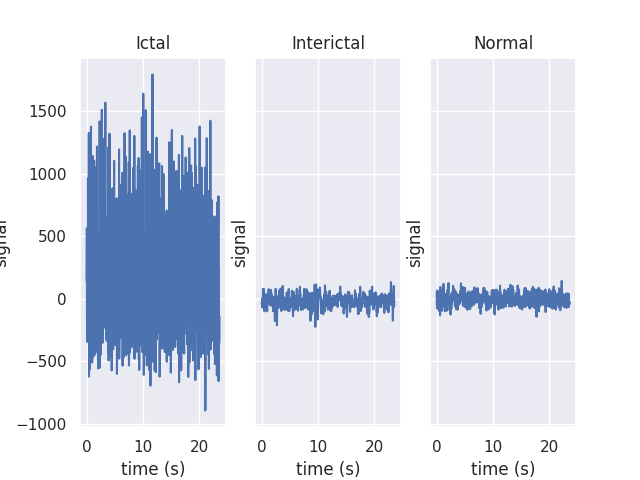
In this example we’ll use the cesium library to compare various techniques for epilepsy detection using a classic EEG time series dataset from Andrzejak et al.. The raw data are separated into five classes: Z, O, N, F, and S; we will consider a three-class classification problem of distinguishing normal (Z, O), interictal (N, F), and ictal (S) signals.

The overall workflow consists of three steps: first, we “featurize” the time series by selecting some set of mathematical functions to apply to each; next, we build some classification models which use these features to distinguish between classes; finally, we validate our models by generating predictions for some unseen holdout set and comparing them to the true class labels.

First, we’ll load the data and inspect a representative time series from each class:

import numpy as np
import matplotlib.pyplot as plt
import seaborn
from cesium import datasets

seaborn.set()

eeg = datasets.fetch_andrzejak()

# Group together classes (Z, O), (N, F), (S) as normal, interictal, ictal
eeg["classes"] = eeg["classes"].astype("U16")  # allocate memory for longer class names
eeg["classes"][np.logical_or(eeg["classes"] == "Z", eeg["classes"] == "O")] = "Normal"
eeg["classes"][
    np.logical_or(eeg["classes"] == "N", eeg["classes"] == "F")
] = "Interictal"
eeg["classes"][eeg["classes"] == "S"] = "Ictal"

fig, ax = plt.subplots(1, len(np.unique(eeg["classes"])), sharey=True)
for label, subplot in zip(np.unique(eeg["classes"]), ax):
    i = np.where(eeg["classes"] == label)[0][0]
    subplot.plot(eeg["times"][i], eeg["measurements"][i])
    subplot.set(xlabel="time (s)", ylabel="signal", title=label)

Downloading data from https://github.com/cesium-ml/cesium-data/raw/main/andrzejak/

Featurization

Once the data is loaded, we can generate features for each time series using the cesium.featurize module. The featurize module includes many built-in choices of features which can be applied for any type of time series data; here we’ve chosen a few generic features that do not have any special biological significance.

By default, the time series will featurized in parallel using the dask.threaded scheduler; other approaches, including serial and distributed approaches, can be implemented by passing in other dask schedulers as the get argument to featurize_time_series.

from cesium import featurize

features_to_use = [
    "amplitude",
    "percent_beyond_1_std",
    "maximum",
    "max_slope",
    "median",
    "median_absolute_deviation",
    "percent_close_to_median",
    "minimum",
    "skew",
    "std",
    "weighted_average",
]
fset_cesium = featurize.featurize_time_series(
    times=eeg["times"],
    values=eeg["measurements"],
    errors=None,
    features_to_use=features_to_use,
)
print(fset_cesium.head())

feature amplitude percent_beyond_1_std  ...        std weighted_average
channel         0                    0  ...          0                0
0           143.5             0.327313  ...  40.411000        -4.132048
1           211.5             0.290212  ...  48.812668       -52.444716
2           165.0             0.302660  ...  47.144789        12.705150
3           171.5             0.300952  ...  47.072316        -3.992433
4           170.0             0.305101  ...  44.910958       -17.999268

[5 rows x 11 columns]

The output of featurize_time_series is a pandas.DataFrame which contains all the feature information needed to train a machine learning model: feature names are stored as column indices (as well as channel numbers, as we’ll see later for multi-channel data), and the time series index/class label are stored as row indices.

Custom feature functions

Custom feature functions not built into cesium may be passed in using the custom_functions keyword, either as a dictionary {feature_name: function}, or as a dask graph. Functions should take three arrays times, measurements, errors as inputs; details can be found in the cesium.featurize documentation. Here we’ll compute five standard features for EEG analysis provided by Guo et al. (2012):

import numpy as np
import scipy.stats


def mean_signal(t, m, e):
    return np.mean(m)


def std_signal(t, m, e):
    return np.std(m)


def mean_square_signal(t, m, e):
    return np.mean(m**2)


def abs_diffs_signal(t, m, e):
    return np.sum(np.abs(np.diff(m)))


def skew_signal(t, m, e):
    return scipy.stats.skew(m)

Now we’ll pass the desired feature functions as a dictionary via the custom_functions keyword argument.

guo_features = {
    "mean": mean_signal,
    "std": std_signal,
    "mean2": mean_square_signal,
    "abs_diffs": abs_diffs_signal,
    "skew": skew_signal,
}

fset_guo = featurize.featurize_time_series(
    times=eeg["times"],
    values=eeg["measurements"],
    errors=None,
    features_to_use=list(guo_features.keys()),
    custom_functions=guo_features,
)
print(fset_guo.head())

feature       mean        std        mean2 abs_diffs      skew
channel          0          0            0         0         0
0        -4.132048  40.411000  1650.122773   46948.0  0.032805
1       -52.444716  48.812668  5133.124725   61118.0 -0.092715
2        12.705150  47.144789  2384.051989   51269.0 -0.004100
3        -3.992433  47.072316  2231.742495   75014.0  0.063678
4       -17.999268  44.910958  2340.967781   52873.0  0.142753

Multi-channel time series

The EEG time series considered here consist of univariate signal measurements along a uniform time grid. But featurize_time_series also accepts multi-channel data; to demonstrate this, we will decompose each signal into five frequency bands using a discrete wavelet transform as suggested by Subasi (2005), and then featurize each band separately using the five functions from above.

import pywt

n_channels = 5
eeg["dwts"] = [
    pywt.wavedec(m, pywt.Wavelet("db1"), level=n_channels - 1)
    for m in eeg["measurements"]
]
fset_dwt = featurize.featurize_time_series(
    times=None,
    values=eeg["dwts"],
    errors=None,
    features_to_use=list(guo_features.keys()),
    custom_functions=guo_features,
)
print(fset_dwt.head())

feature        mean                      ...      skew
channel           0         1         2  ...         2         3         4
0        -17.080739 -6.067121 -0.979336  ...  0.299892  0.123948  0.117937
1       -210.210117 -3.743191  0.511377  ...  0.168179 -0.005521  0.187815
2         51.831712  0.714981  0.247418  ... -0.254241 -0.061304 -0.136422
3        -15.429961  9.348249 -0.099243  ... -0.013705 -0.007339  0.013836
4        -71.982490 -3.787938 -0.183324  ...  0.285906  0.087555  0.066677

[5 rows x 25 columns]

The output featureset has the same form as before, except now the channel component of the column index is used to index the features by the corresponding frequency band.

Model Building

Featuresets produced by cesium.featurize are compatible with the scikit-learn API. For this example, we’ll test a random forest classifier for the built-in cesium features, and a 3-nearest neighbors classifier for the others, as suggested by Guo et al. (2012).

from sklearn.ensemble import RandomForestClassifier
from sklearn.neighbors import KNeighborsClassifier
from sklearn.model_selection import train_test_split

train, test = train_test_split(np.arange(len(eeg["classes"])), random_state=0)

model_cesium = RandomForestClassifier(n_estimators=128, random_state=0)
model_cesium.fit(fset_cesium.iloc[train], eeg["classes"][train])

model_guo = KNeighborsClassifier(3)
model_guo.fit(fset_guo.iloc[train], eeg["classes"][train])

model_dwt = KNeighborsClassifier(3)
model_dwt.fit(fset_dwt.iloc[train], eeg["classes"][train])

KNeighborsClassifier(n_neighbors=3)

In a Jupyter environment, please rerun this cell to show the HTML representation or trust the notebook.
On GitHub, the HTML representation is unable to render, please try loading this page with nbviewer.org.

Prediction

Making predictions for new time series based on these models follows the same pattern: first the time series are featurized using featurize_time_series, and then predictions are made based on these features using the predict method of the scikit-learn model.

from sklearn.metrics import accuracy_score

preds_cesium = model_cesium.predict(fset_cesium)
preds_guo = model_guo.predict(fset_guo)
preds_dwt = model_dwt.predict(fset_dwt)

print(
    "Built-in cesium features: training accuracy={:.2%}, test accuracy={:.2%}".format(
        accuracy_score(preds_cesium[train], eeg["classes"][train]),
        accuracy_score(preds_cesium[test], eeg["classes"][test]),
    )
)
print(
    "Guo et al. features: training accuracy={:.2%}, test accuracy={:.2%}".format(
        accuracy_score(preds_guo[train], eeg["classes"][train]),
        accuracy_score(preds_guo[test], eeg["classes"][test]),
    )
)
print(
    "Wavelet transform features: training accuracy={:.2%}, test accuracy={:.2%}".format(
        accuracy_score(preds_dwt[train], eeg["classes"][train]),
        accuracy_score(preds_dwt[test], eeg["classes"][test]),
    )
)

Built-in cesium features: training accuracy=100.00%, test accuracy=83.20%
Guo et al. features: training accuracy=92.80%, test accuracy=83.20%
Wavelet transform features: training accuracy=97.87%, test accuracy=95.20%

The workflow presented here is intentionally simplistic and omits many important steps such as feature selection, model parameter selection, etc., which may all be incorporated just as they would for any other scikit-learn analysis. But with essentially three function calls (featurize_time_series, model.fit, and model.predict), we are able to build a model from a set of time series and make predictions on new, unlabeled data. In upcoming posts we’ll introduce the web frontend for cesium and describe how the same analysis can be performed in a browser with no setup or coding required.